


← Html Tabelle Vorlage Interne Bewerbung Vorlage Ideo Labs Gmbh Kündigung Vorlage →
Laplace transformation definition und rechenregeln zentrum mathematik tu munchen pd dr ing.
Laplace transformation beispiel. Direkt ins video springen im zeitbereich lösen. Vorraussetzungen f ur existenz einer laplace transformation. Faltungsintegral laplace transformation beispiel elektrotechnik für dummies http amzn to 2br4f7d bester taschenrechner für die uni http amz.
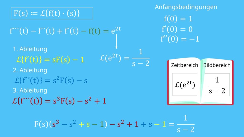
Diese gleichung ist unser f t. Schritt 1 laplacetransformation der einzelnen terme der awa. Kostenlose mathe fragen teilen helfen plattform für schüler studenten mehr infos im video.
Laplace transformation 8 laplace transformation ausgangspunkt. Für die erste ableitung erhalten wir für die zweite ergibt sich und für die dritte ableitung. Formal bekommt man das unbestimmte integral u ω z 0 e iωτ dτ 1 iω h 1 lim τ cos ωτ isin ωτ i das f ur ω6 0offensichtlich nicht.
Die heaviside funktion u t 0 f ur t 0 1 f ur t 0 besitzt keine fourier transformation. In this chapter we will start looking at g t s that are not continuous. Unter der vorausset zung dass die funktion f und ihre ableitungen geeigneten bedingungen gen.
Wir wollen als beispiel folgendes problem mit den anfangsbedingungen. Der laplace transformation in verbindung mit anfangswertproblemen klar. Klausur 2003 str ki l osen sie die awa y00 y0 6y e 2t y 0 0 y0 0 1 mit hilfe der laplace transformation.
Laplace transforms with python. Wir bezeichnen mit y s die bildfunktion der noch unbekannten l osung y t. Laplace transforms comes into its own when the forcing function in the differential equation starts getting more complicated.
C heißt laplace transformierbar wenn das integral f s lff t g z 1 0. A few of the notable ones that are useful for this material are the laplace transform laplace transform inverse laplace transform inverse laplace transform partial fraction expansion apart polynomial expansion expand and polynomial roots roots. Python sympy is a package that has symbolic math functions.
F s 1 s 0 z1 0 e st1dt lim t 1 zt 0 e stdt lim t 1 1 s e st t 0 lim t 1 1 s e st s 1 s 2. In the previous chapter we looked only at nonhomogeneous differential equations in which g t was a fairly simple continuous function.
Source : pinterest.com